Exploratory Data Analysis (EDA) of the 2022 Commonwealth Games

Continuing my learning journey of Python (and tools) in data analysis, there was a data set for the 2022 Commonwealth Games.  I thought that since I had just done some EDA on the Olympics, it would be good to look at this data set.

So, let's begin...

import pandas as pd
import numpy as np
import matplotlib.pyplot as plt
%matplotlib inline
import matplotlib.patches as mpatches
from matplotlib.pyplot import figure
import matplotlib.mlab as mlab
import scipy.stats
import seaborn as sns
sns.set_theme(style='whitegrid', font_scale=1.5)

players_raw = pd.read_csv('/content/drive/MyDrive/Colab Notebooks/Commonwealth 2022/commonwealth games 2022 - players participated.csv')
winners_raw = pd.read_csv('/content/drive/MyDrive/Colab Notebooks/Commonwealth 2022/commonwealth games 2022 - players won medals in cwg games 2022.csv')
medal_tally = pd.read_csv('/content/drive/MyDrive/Colab Notebooks/Commonwealth 2022/MEDAL TALLY.csv')

#Players names in the 'players.csv' file have their firstname and surname joined together without a space, so let's fix that:
players_raw['athlete_name'] = players_raw['athlete_name'].str.replace( r"([A-Z])", r" \1", regex=True).str.strip()

# I wanted to add the athlete's age and gender into the winners dataset.  I've probably done this a long-winded way, but I've done it without inPlace=True, and utilised the pd.merge function
winners2 = pd.merge(winners_raw, players_raw, on="athlete_name", how="left")
winners3 = winners2[
    [
        "athlete_name",
        "team_x",
        "sport_x",
        "event",
        "medal",
        "region_x",
        "event_type",
        "gender",
        "age",
    ]
]
winners = winners3.rename(
    columns={"sport_x": "sport", "team_x": "team", "region_x": "region"}
)
winners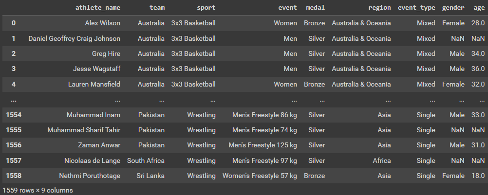

#The 'players' table didn't include medalling information so I've brought that in via the other csv file.  
#I did do a little clean up within the CSV to ensure that data integrity and validation could more easily be done.
players = pd.merge(players_raw, winners, on="athlete_name", how="left")
players = players[
    ["athlete_name", "sport_x", "gender_x", "team_x", "medal", "age_x", "region_x"]
]
players = players.rename(
    columns={
        "sport_x": "sport",
        "team_x": "team",
        "gender_x": "gender",
        "age_x": "age",
        "region_x": "region",
        "medal": "medalled"
    }
)
players[['medalled']] = players[['medalled']].fillna('None')
players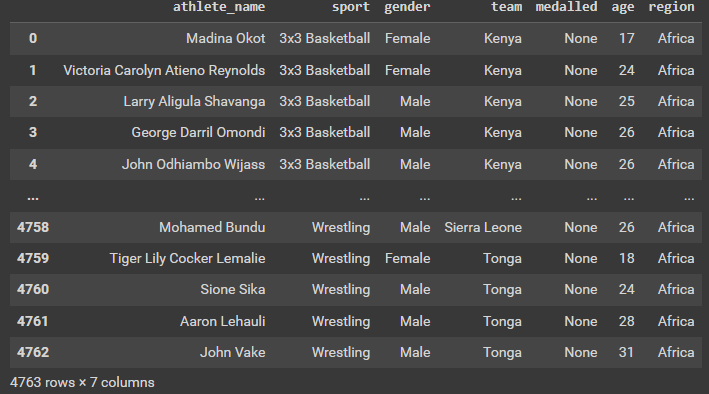

plt.figure(figsize = (14,8))
players_age_by_gender = sns.histplot(data=players, x='age', hue='gender', binwidth=1, palette={"Male": "b", "Female": "hotpink"})
plt.ylabel('NUMBER OF ATHLETES')
plt.xlabel('AGE')
plt.suptitle('Number of Athletes by age & Gender', x=0.33, y=0.92)
sns.despine(top=True, right=True, left=False, bottom=False, offset=None, trim=False)
plt.xlim(0, 80)
plt.ylim(0, 250)
plt.show()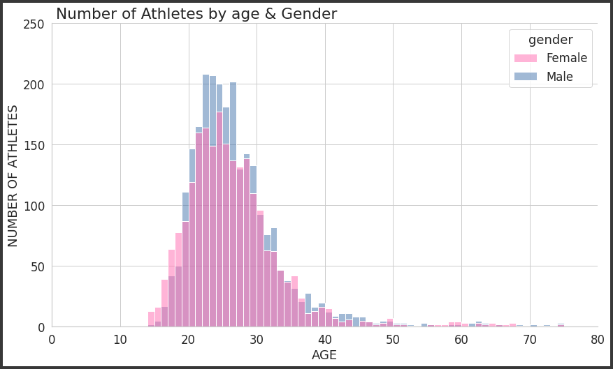

plt.figure(figsize = (14,8))
winners_age_by_gender = sns.histplot(data=winners, x='age', hue='gender', binwidth=1, palette={"Male": "b", "Female": "hotpink"})
plt.ylabel('NUMBER OF MEDALISTS')
plt.xlabel('AGE')
plt.suptitle('Number of Medalists by Age & Gender', x=0.33, y=0.92)
sns.despine(top=True, right=True, left=False, bottom=False, offset=None, trim=False)
plt.xlim(0, 80)
plt.ylim(0, 60)
plt.show()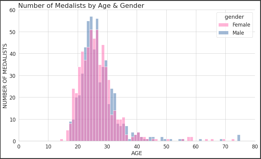

I thought it would be interesting to have a quick look at the age splits based on the most energetic sport (athletics) compared to the least physically strenuous.  For this, I decided to look specifically at Athletics and Lawn Bowls.

bowls_vs_athletics_players = players.loc[players['sport'].isin(['Athletics and Para Athletics','Lawn Bowls and Para Lawn Bowls'])]
bowls_vs_athletics_players[['medalled']] = bowls_vs_athletics_players[['medalled']].fillna('None')
bowls_vs_athletics_players.head()

plt.figure(figsize = (12,6))
players_by_age = sns.histplot(data=bowls_vs_athletics_players, x='age', hue='sport', fill='true', palette={"Athletics and Para Athletics": "b", "Lawn Bowls and Para Lawn Bowls": "g"})
plt.ylabel('NUMBER OF ATHLETES')
plt.xlabel('AGE')
plt.suptitle('Number of Athletes by age - Athletics vs. Lawn Bowls', x=0.46, y=0.96)
plt.xlim(0, 80)
plt.ylim(0, 180)
plt.show()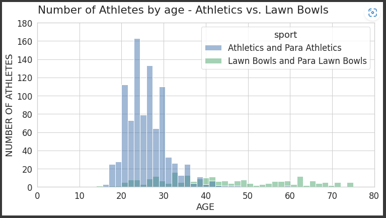

The above shows clearly that the different between Athletics and Bowls. It shows that Bowls is played at top level competition by a wide spread of different ages when compared to Athletics where the majority of athletes are in their 20s.

plt.figure(figsize=(16, 12))
sns.boxplot(y="sport", x="age", data=players)
sns.despine(offset=10, trim=True)
plt.xlim(0, 80)
plt.ylabel("SPORT")
plt.xlabel("AGE")
plt.suptitle("Age Range per Sport", x=0.24, y=0.94)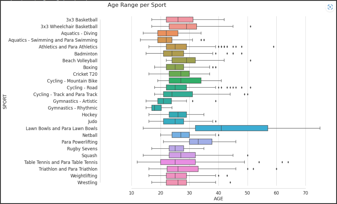

plt.figure(figsize=(12, 14))
players_age_by_gender = sns.histplot(
    data=players,
    y="sport",
    hue="gender",
    multiple="dodge",
    shrink=0.8,
    palette={"Male": "b", "Female": "hotpink"},
)
plt.xticks(rotation=90)
sns.despine(offset=10, trim=True)
plt.ylabel("SPORT")
plt.xlabel("Number of Athletes")
plt.suptitle("Number of Athletes per Sport by Gender", x=0.4, y=0.9)
plt.show()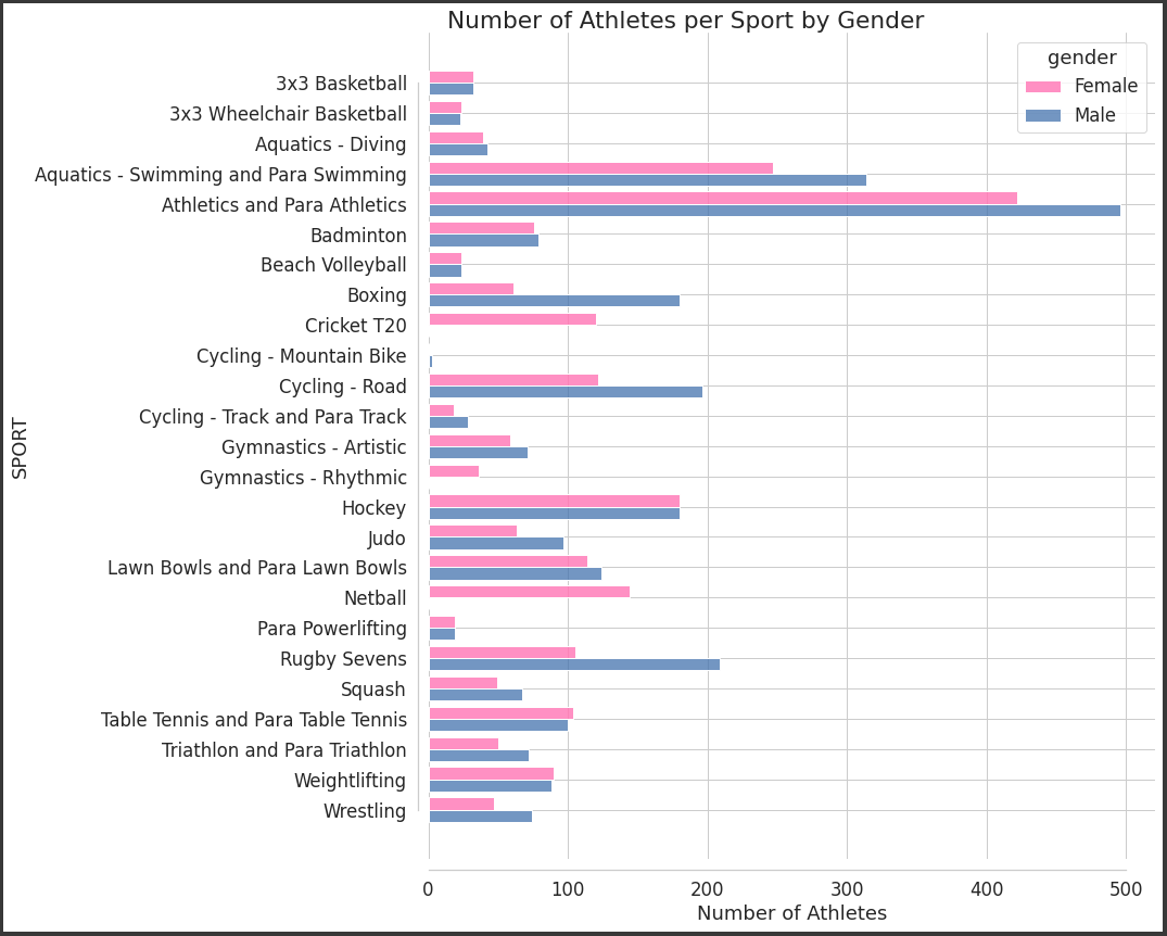

plt.figure(figsize=(14, 12))
sns.violinplot(
    data=players2,
    y="region_x",
    x="age_x",
    hue="gender_x",
    split=True,
    inner="quart",
    linewidth=1,
    palette={"Male": "b", "Female": "hotpink"},
    bw=0.1,
    scale="count",
    cut=0,
)
plt.xlim(0, 80)
sns.despine(left=True)
plt.legend(title="Gender", loc="upper right")
plt.ylabel("REGION")
plt.xlabel("AGE")
plt.suptitle("Age Profile of Athletes per Region by Gender", x=0.38, y=0.95)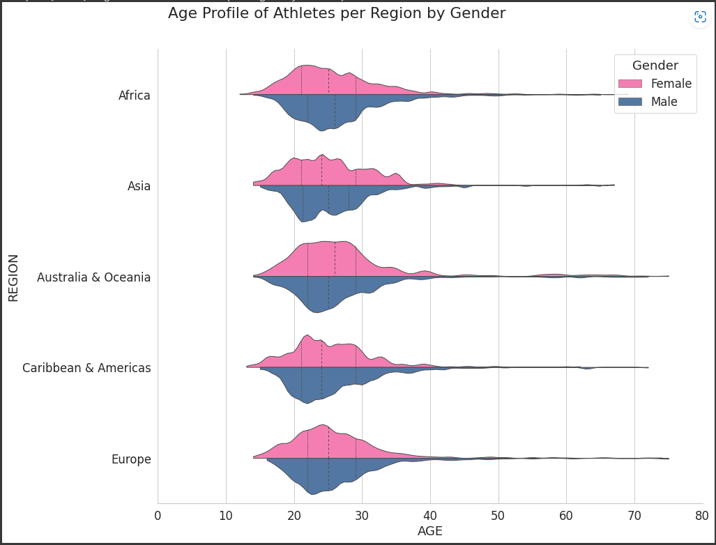

That's it for part one.  I am working on some exploratory data analysis for the medals which I will publish in the future as a part 2 to this.

Pete

❤️ Enjoyed this article?

Forward to a friend and let them know where they can subscribe (hint: it's here).