
Continuing on my journey through Python and given that we've just had Hallowe'en, I thought it'd be a good idea to find an appropriate dataset. The dataset is from the TidyTuesday GitHub and can be found here: https://github.com/rfordatascience/tidytuesday/tree/master/data/2022/2022-11-01
Data set was extracted from The Movie Database via the tmdb API using R httr. There are ~35K movie records in this dataset.
Let's load in the tools that we'll need for this EDA:
import pandas as pd
import numpy as np
import matplotlib.pyplot as plt
%matplotlib inline
import calendar
import matplotlib.patches as mpatches
from matplotlib.pyplot import figure
import matplotlib.mlab as mlab
import seaborn as sns
sns.set_theme(style='whitegrid', font_scale=1.5)
# Reading in the data
data = pd.read_csv('/horror_movies.csv', encoding="ISO-8859-1")Beforehand, I had opened the data in Excel to add a couple of columns that might prove useful. I've added the columns: language, release_month, release_q, decade, budget_range, cpi_month, and cpi_value.
I thought I would add CPI values to analyse the revenue and budgets of films where we shouldn't solely rely on nominal values because inflation will significatly warp the data due to the 70 year range we're looking at.
I noticed that the revenue and budget figures were large numbers so thought it's best to roll it up into millions. We're also going to add release_year to the data.
data["revenue($m)"] = data["revenue"] / 1000000
data["budget($m)"] = data["budget"] / 1000000
hf = data[
    [
        "id",
        "title",
        "language",
        "release_date",
        "release_month",
        "decade",
        "popularity",
        "vote_count",
        "vote_average",
        "revenue",
        "profit_pct",
        "budget",
        "revenue($m)",
        "budget($m)",
        "runtime",
        "status",
        "cpi_index"
    ]
]
hf["release_date"] = pd.to_datetime(hf["release_date"])
hf['release_year'] = pd.DatetimeIndex(hf['release_date']).year
hf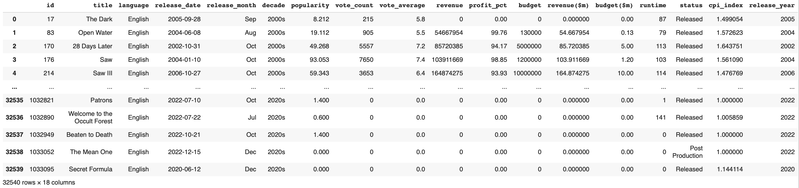
Let's initially see how many films are being released per year:
plt.figure(figsize=(14, 8))
ax = sns.histplot(data=hf, x="release_year")

plt.gca().spines["top"].set_visible(False)
plt.gca().spines["right"].set_visible(False)
plt.ylabel("NUMBER OF FILMS RELEASED", y=0.35)
plt.xlabel("YEAR")
plt.suptitle("Number of Horror Films Released per Year Since 1950", x=0.42)
plt.figtext(0.9, 0.0, "Data Source: shorturl.at/clzE2", horizontalalignment="right", fontsize=10)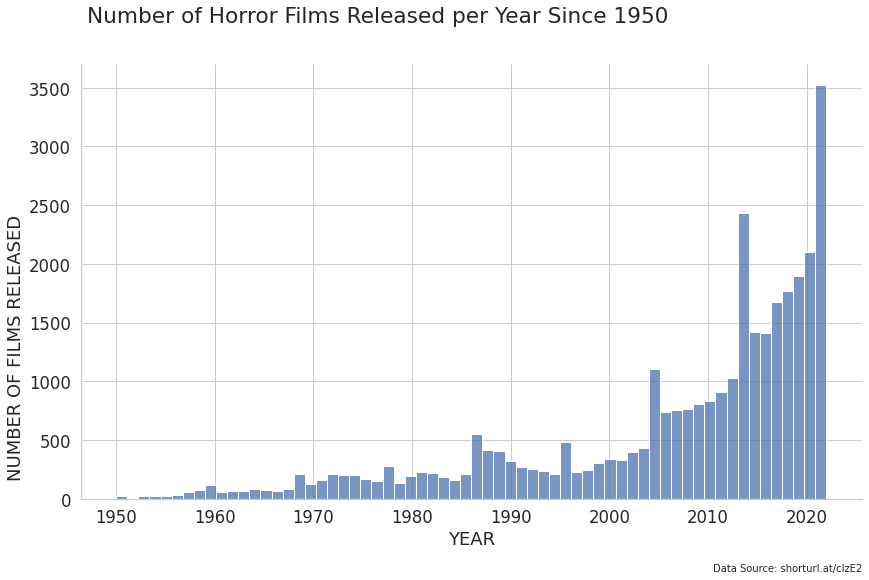
I want to have a look at which months films are released in so we should make a dataframe to hold that data. Below, we are firstly sorting the values by release_date, grouping them by the release year, and then sorting them in month order. I needed to make a separate dataframe to ensure that the months were in chronological order.
films_month = hf.sort_values('release_date')
films_month = films_month.groupby('release_month')['release_month'].count().reset_index(name="films_released")


month_order = {'Jan':1,'Feb':2,'Mar':3, 'Apr':4, 'May':5, 'Jun':6, 'Jul':7, 'Aug':8, 'Sep':9, 'Oct':10, 'Nov':11, 'Dec':12}

films_month = films_month.sort_values('release_month', key = lambda x : x.apply (lambda x : month_order[x]))
films_month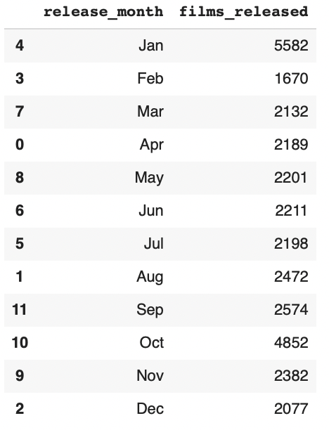
Now with the data prepped, lets visualise this in a chart:
plt.figure(figsize=(14, 8))
ax = sns.barplot(data=films_month, x="release_month", y="films_released")

for bar in ax.patches:
    if bar.get_height() > 3000:
        bar.set_color("darkred")
    else:
        bar.set_color("grey")

plt.gca().spines["top"].set_visible(False)
plt.gca().spines["right"].set_visible(False)
plt.ylabel("NUMBER OF FILMS RELEASED", y=0.35)
plt.xlabel("MONTH", x=0.05)
plt.suptitle("Number of Horror Films Released per Month Since 1950", x=0.42)
plt.figtext(0.9, 0.0, "Data Source: shorturl.at/clzE2", horizontalalignment="right", fontsize=10)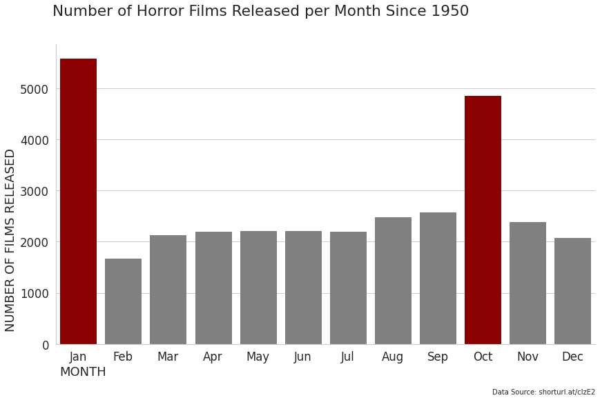
It is clear to see that the months of January and October are the most popular for releasing a horror film - it goes to show the impact of Hallowe'en.
I have noticed that Hallowe'en is beomcing a more popular time of the year so I wonder if this month release trend has changed over time. Let's plot the above but over the year range we have in the data.
jan_v_oct = hf.loc[hf['release_month'].isin(['Jan','Oct'])]

plt.figure(figsize=(14, 8))

ax = sns.histplot(data=jan_v_oct, x="release_year", hue="release_month", hue_order=['Oct', 'Jan'])

plt.gca().spines["top"].set_visible(False)
plt.gca().spines["right"].set_visible(False)
plt.ylabel("NUMBER OF FILMS RELEASED", y=0.35)
plt.xlabel("YEAR")
plt.legend(title='Month', loc='upper left', labels=['January', 'October'])
plt.suptitle("Comparing Films Released in January & October", x=0.42)
plt.figtext(0.9, 0.0, "Data Source: shorturl.at/clzE2", horizontalalignment="right", fontsize=10)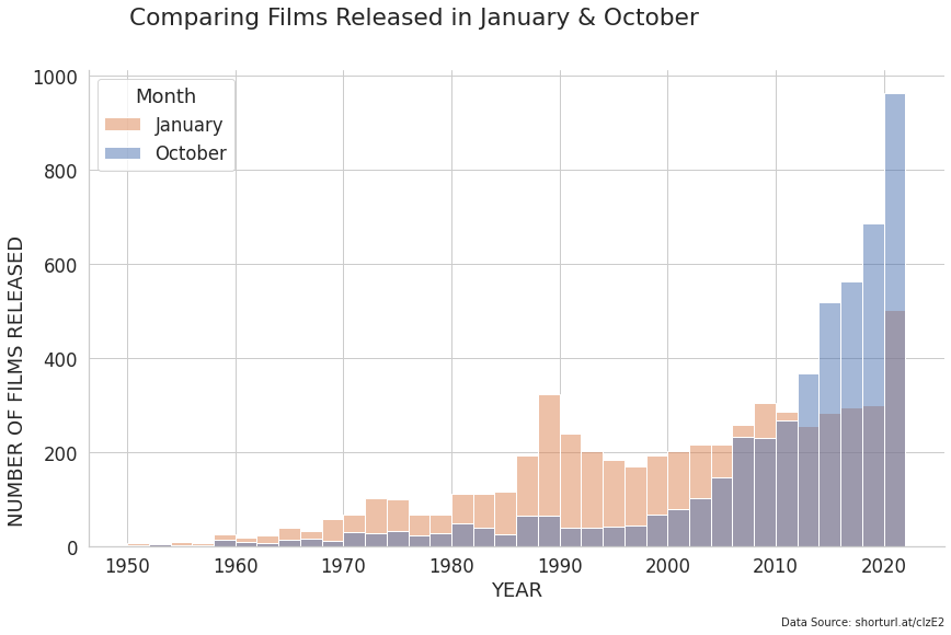
I think it is insightful that this graph shows a transition from January being the most popular release month during the 1970s up til the early 2000s, but there's been a shift in the last 20 years where October has become the most popular month and has exponentially grown as the most popular release month.
Let's adjust the revenue and budget amounts to account for inflation. I have used the CPI data from FRED here: https://fred.stlouisfed.org/series/CPIAUCNS
hf['CPIAdjrevenue'] = hf['revenue($m)'] * hf['cpi_index']
hf['CPIAdjbudget'] = hf['budget($m)'] * hf['cpi_index']
#Create a way of showing data labels for either horizontal or vertical graphs
def show_values(axs, orient="v", space=.01):
def _single(ax):
if orient == "v":
for p in ax.patches:
_x = p.get_x() + p.get_width() / 2
_y = p.get_y() + p.get_height() + (p.get_height()*0.01)
value = '{:.1f}'.format(p.get_height())
ax.text(_x, _y, value, ha="center")
elif orient == "h":
for p in ax.patches:
_x = p.get_x() + p.get_width() + float(space)
_y = p.get_y() + p.get_height() - (p.get_height()*0.5)
value = '{:.1f}'.format(p.get_width())
ax.text(_x, _y, value, ha="left")
if isinstance(axs, np.ndarray):
for idx, ax in np.ndenumerate(axs):
_single(ax)
else:
_single(axs)#Load the dataset
top10_revenue = hf.sort_values('CPIAdjrevenue', ascending=False).head(10)
#Initialise the matplotlib figure
plt.figure(figsize=(14, 8))
#Plot the revenue amount
sns.set_color_codes("pastel")
ax = sns.barplot(data=top10_revenue, x="CPIAdjrevenue", y="title", label="Revenue($m)", color="r")
show_values(ax, "h", space=0)
#Plot the budget amount
sns.set_color_codes("muted")
ax = sns.barplot(data=top10_revenue, x="CPIAdjbudget", y="title", label="Budget($m)", color="r")
show_values(ax, "h", space=0)
#Add grapgh information ie. titles, legend, data labels, etc
plt.gca().spines["top"].set_visible(False)
plt.gca().spines["right"].set_visible(False)
plt.ylabel("Film Title")
plt.xlabel("CPI Adjusted Revenue ($m)")
plt.suptitle("Top 10 Biggest Revenue ($m) Generating Films (CPI Adjusted)", x=0.42)
ax.legend(loc="lower right", frameon=True)
plt.figtext(0.9, -0.0, "Data Source: shorturl.at/clzE2", horizontalalignment="right", fontsize=10)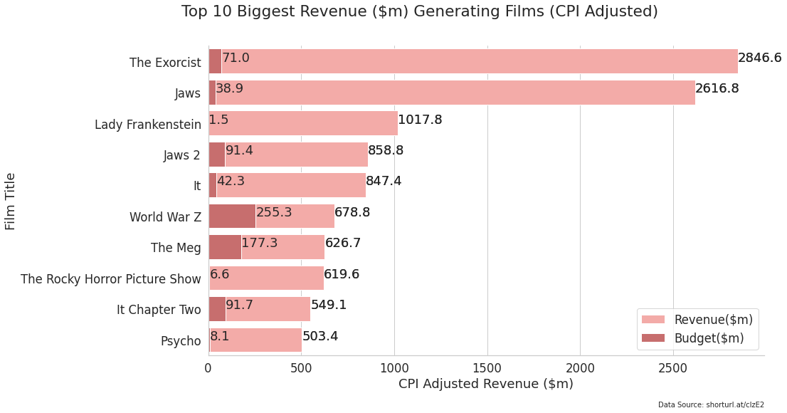
#Top 25 highest rated films where vote count was more than 1000
rating_top20 = hf[hf['vote_count'] > 1000].sort_values(by='vote_average', ascending=False).head(20)

#Initialise the matplotlib figure
plt.figure(figsize=(10, 12))

#Plot the revenue amount
sns.set_color_codes("muted")
ax = sns.barplot(data=rating_top20, x="vote_average", y="title", label="vote_average", color="r")
show_values(ax, "h", space=0)

#Add graph information ie. titles, legend, data labels, etc
plt.gca().spines["top"].set_visible(False)
plt.gca().spines["right"].set_visible(False)
plt.ylabel("Film Title")
plt.xlabel("Vote Score (out of 10)")
plt.suptitle("Top 10 All Time Horror Films (where Vote Count >1000)")
plt.figtext(0.9, 0.0, "Data Source: shorturl.at/clzE2", horizontalalignment="right", fontsize=10)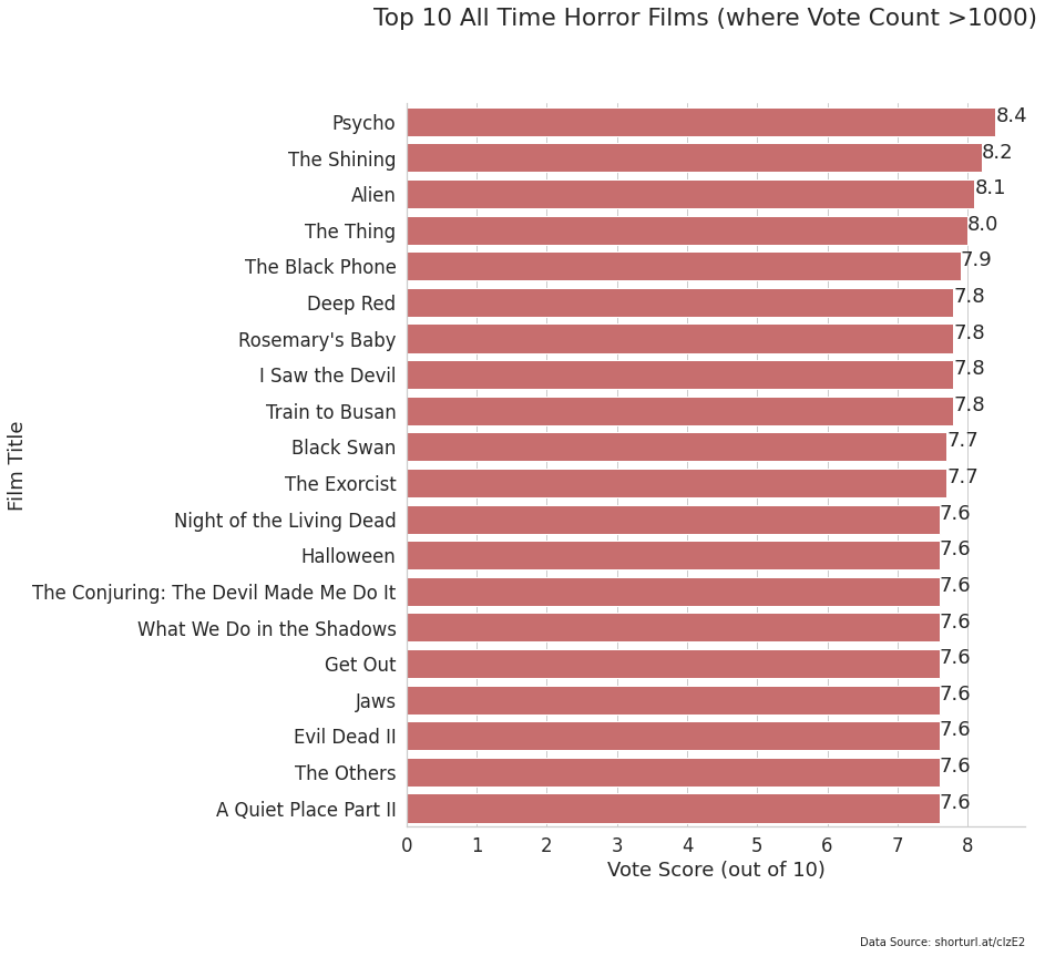
plt.figure (figsize = (18,12))
sns.set_style('ticks')

corr = hf.corr()

sns.heatmap (data = corr, annot=True, cmap='coolwarm', fmt='.2f', linewidth = 1)
sns.set (font_scale = 0)
plt.show ()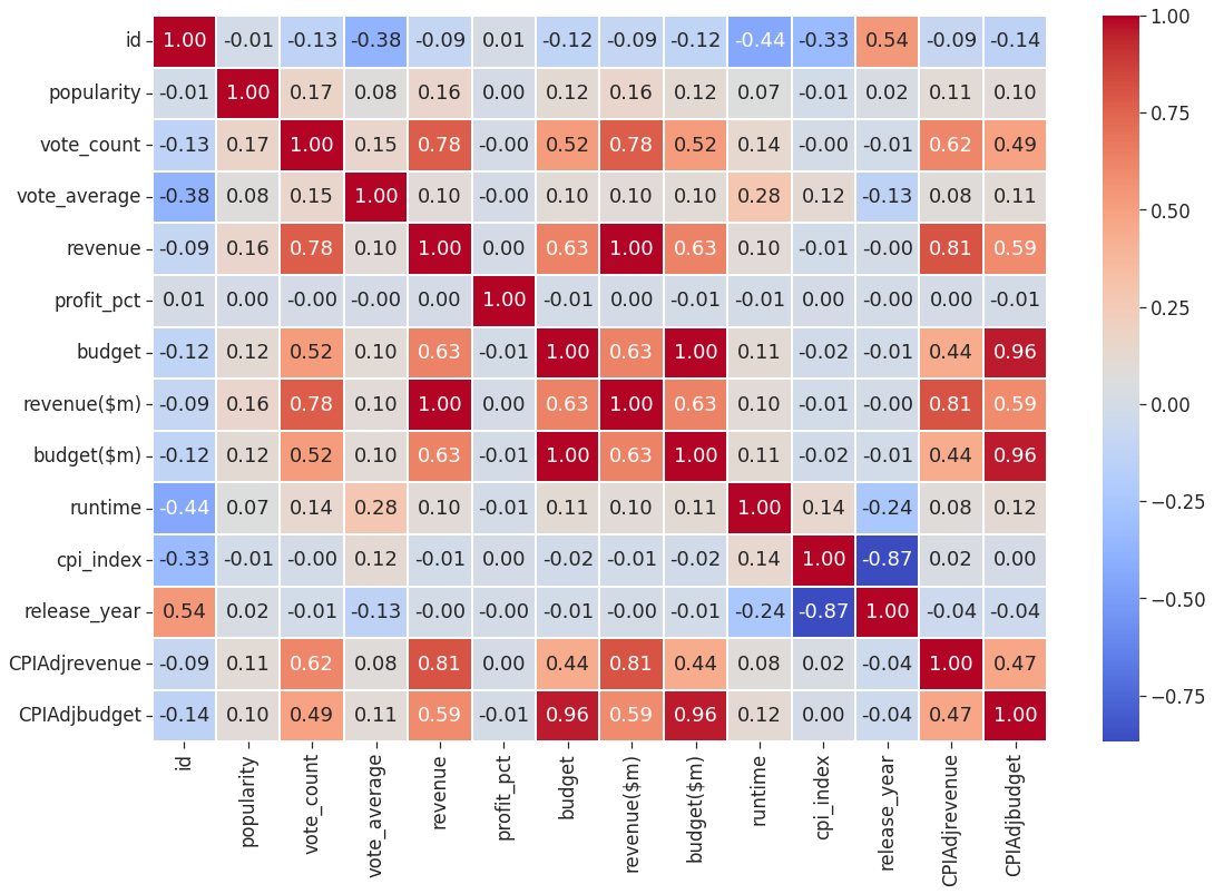
The above heatmap is to see if there's any standout positive or negative correlations in the data. There's a strong positive correlation between revenue generated and amount of votes (0.78) which shows that higher earning films also attract the most votes. There's also a positive correlation between the amount of budget for a film and the revenue it generates (0.63).
The amount of profit margin made is most positively affected by the average vote count.
The other interesting point is that there's a slight negative correlation between release year and vote average - does this mean that viewers feel that horror films are getting worse over time?
There's also a slight negative correlation between release year and runtime which may suggest that films are getting shorter.
hf_ratings = hf[hf['vote_count'] > 50]

plt.figure(figsize=(18, 8))
ax = sns.boxplot(data=hf_ratings, x="release_year", y="vote_average")

plt.gca().spines["top"].set_visible(False)
plt.gca().spines["right"].set_visible(False)
plt.xticks(rotation=45)
every_nth = 5
for n, label in enumerate(ax.xaxis.get_ticklabels()):
    if n % every_nth != 0:
        label.set_visible(False)
plt.ylabel("AVERAGE VOTE COUNT", y=0.35)
plt.xlabel("YEAR")
plt.suptitle("Average Vote of Films per Year")
plt.figtext(0.9, 0.0, "Data Source: shorturl.at/clzE2", horizontalalignment="right", fontsize=10)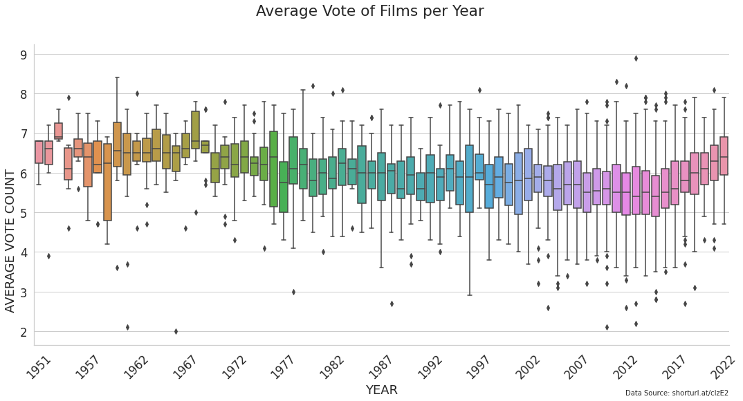
Interestingly, it looks like horror films have been slowly declining in vote average since the early 1960s until around 2016 when they have started to increase in vote score quite quickly. Is there a resurgence in this genre of films?
❤️ Enjoyed this article?
Forward to a friend and let them know where they can subscribe (hint: it's here).


